Machine Learning [Week 03/11] Logistic Regression

[mathjax]

Machine Learning (Stanford University) の受講メモ

Classification and Representation

Classification

To attempt classification, one method is to use linear regression and map all predictions greater than 0.5 as a 1 and all less than 0.5 as a 0. However, this method doesn’t work well because classification is not actually a linear function.

The classification problem is just like the regression problem, except that the values we now want to predict take on only a small number of discrete values. For now, we will focus on the binary classification problem in which y can take on only two values, 0 and 1. (Most of what we say here will also generalize to the multiple-class case.) For instance, if we are trying to build a spam classifier for email, then \(x^{(i)}\) may be some features of a piece of email, and y may be 1 if it is a piece of spam mail, and 0 otherwise. Hence, y∈{0,1}. 0 is also called the negative class, and 1 the positive class, and they are sometimes also denoted by the symbols “-” and “+.” Given \(x^{(i)}\), the corresponding \(y^{(i)}\) is also called the label for the training example.

(note)

• \(y\in\{0,1\}\)
  • 0: Negative Class
  • 1: Positive Class
• Threshold classifier output \(h_\theta(x)\) at 0.5:$$
  \text{If }h_\theta(x)\geq 0.5, \text{ predict }”y=1″\\
  \text{If }h_\theta(x)\lt 0.5, \text{ predict }”y=0″\\
  $$

Hypothesis Representation

We could approach the classification problem ignoring the fact that y is discrete-valued, and use our old linear regression algorithm to try to predict y given x. However, it is easy to construct examples where this method performs very poorly. Intuitively, it also doesn’t make sense for \(h_\theta (x)\) to take values larger than 1 or smaller than 0 when we know that y ∈ {0, 1}. To fix this, let’s change the form for our hypotheses \(h_\theta (x)\) to satisfy \(0 \leq h_\theta (x) \leq 1\). This is accomplished by plugging \(\theta^Tx\) into the Logistic Function.

Our new form uses the “Sigmoid Function,” also called the “Logistic Function”:

\[
\begin{align}& h_\theta (x) = g ( \theta^T x ) \newline \newline& z = \theta^T x \newline& g(z) = \dfrac{1}{1 + e^{-z}}\end{align}
\]

The following image shows us what the sigmoid function looks like:

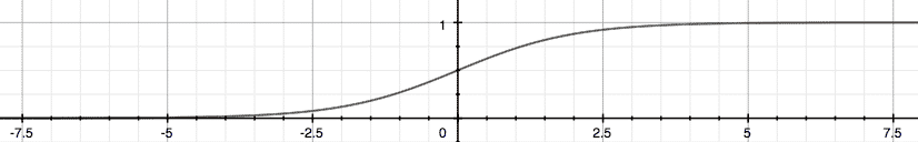
The function g(z), shown here, maps any real number to the (0, 1) interval, making it useful for transforming an arbitrary-valued function into a function better suited for classification.

\(h_\theta(x)\) will give us the probability that our output is 1. For example, \(h_\theta(x)=0.7\) gives us a probability of 70% that our output is 1. Our probability that our prediction is 0 is just the complement of our probability that it is 1 (e.g. if probability that it is 1 is 70%, then the probability that it is 0 is 30%).

\[
\begin{align}& h_\theta(x) = P(y=1 | x ; \theta) = 1 – P(y=0 | x ; \theta) \newline& P(y = 0 | x;\theta) + P(y = 1 | x ; \theta) = 1\end{align}
\]

(note)

• Logistic Regression Model
  • \(\text{Want }0\leq h_\theta(x) \leq 1\)
    \[
    h_\theta(x)=g(\theta^Tx)=g(z)=\frac{1}{1+e^{-z}}=\frac{1}{1-e^{-\theta^Tx}}
    \]
  • g function
    • Sigmoid function same as Logistic function
• Interpretation of Hypothesis Output
  • \(h(x)\)=estimated probability that y=1 on input x
  • Example: If\[
    x=\begin{bmatrix}
    x_0\\
    x_1
    \end{bmatrix}
    = \begin{bmatrix}
    1\\
    tumorSize
    \end{bmatrix}
    \]
  • \[
    h_\theta(x)=P(y=1|x;\theta)\\
    y=0 or 1
    \]
  • probability that y = 1, given x, parameterized by \(\theta\)
  • \[
    P(y=0|x;\theta)+P(y=1|x;\theta)=1\\
    P(y=0|x;\theta)=1-P(y=1|x;\theta)
    \]

Decision Boundary

In order to get our discrete 0 or 1 classification, we can translate the output of the hypothesis function as follows:

\[
\begin{align}& h_\theta(x) \geq 0.5 \rightarrow y = 1 \newline& h_\theta(x) < 0.5 \rightarrow y = 0 \newline\end{align}
\]

The way our logistic function g behaves is that when its input is greater than or equal to zero, its output is greater than or equal to 0.5:

\[
\begin{align}& g(z) \geq 0.5 \newline& when \; z \geq 0\end{align}
\]

Remember.

\[
\begin{align}z=0, e^{0}=1 \Rightarrow g(z)=1/2\newline z \to \infty, e^{-\infty} \to 0 \Rightarrow g(z)=1 \newline z \to -\infty, e^{\infty}\to \infty \Rightarrow g(z)=0 \end{align}
\]

So if our input to g is \(\theta^T X\), then that means:

\[
\begin{align}& h_\theta(x) = g(\theta^T x) \geq 0.5 \newline& when \; \theta^T x \geq 0\end{align}
\]

From these statements we can now say:

\[
\begin{align}& \theta^T x \geq 0 \Rightarrow y = 1 \newline& \theta^T x < 0 \Rightarrow y = 0 \newline\end{align}
\]

The decision boundary is the line that separates the area where y = 0 and where y = 1. It is created by our hypothesis function.

Example:

\[
\begin{align}& \theta = \begin{bmatrix}5 \newline -1 \newline 0\end{bmatrix} \newline & y = 1 \; if \; 5 + (-1) x_1 + 0 x_2 \geq 0 \newline & 5 – x_1 \geq 0 \newline & – x_1 \geq -5 \newline& x_1 \leq 5 \newline \end{align}
\]

In this case, our decision boundary is a straight vertical line placed on the graph where \(x_1 = 5\), and everything to the left of that denotes y = 1, while everything to the right denotes y = 0.

Again, the input to the sigmoid function g(z) (e.g. \(\theta^T X\)) doesn’t need to be linear, and could be a function that describes a circle (e.g. \(z = \theta_0 + \theta_1 x_1^2 +\theta_2 x_2^2\)) or any shape to fit our data.

(note)

• Logistic regression
  • $$
    h_\theta(x)=g(\theta^Tx)\\
    g(z)=\frac{1}{1+e^{-z}}
    $$
• Discrete 0 or 1 classification
  • $$
    \begin{align}
    & h_\theta(x) \geq 0.5 \rightarrow y = 1 \newline
    & h_\theta(x) < 0.5 \rightarrow y = 0 \newline\end{align}
    $$
  • $$
    \begin{align*}
    & g(z) \geq 0.5 \newline
    & when \; z \geq 0\end{align*}
    $$
  • $$
    \begin{align}
    z=0, e^{0}=1 \Rightarrow g(z)=\frac12\newline
    z \to \infty, e^{-\infty} \to 0 \Rightarrow g(z)=1 \newline
    z \to -\infty, e^{\infty}\to \infty \Rightarrow g(z)=0 \end{align}
    $$
  • input to g is \(\theta^TX\)
  • $$
    \begin{align*}
    & h_\theta(x) = g(\theta^T x) \geq 0.5 \newline
    & when \; \theta^T x \geq 0\end{align*}
    $$
  • $$
    \begin{align*}
    & \theta^T x \geq 0 \Rightarrow y = 1 \newline
    & \theta^T x < 0 \Rightarrow y = 0 \newline\end{align*}
    $$
• Decision Boundary
  • \[
    h_\theta(x)=g(\theta_0+\theta_1x_1+\theta_2x_2)
    \]
  • Predict $$
    “y=1” \text{ if } -3+x_1+x_2\geq0
    $$
  • Decision Boundary $$
    x_1+x_2=3
    $$
• Non-linear decision boundaries
  • $$
    h_\theta(x)=g(\theta_0+\theta_1x_1+\theta_2x_2+\theta_3x_1^2+\theta_4x_2^2)\geq 0
    $$
  • Predict $$
    “y=1” \text{ if } -1+x_1^2+x_2^2\geq 0
    $$
  • Decision Boundary $$
    x_1^2+x_2^2= 1
    $$

Logistic Regression Model

• How to choose parameters \(\theta\) ?
  • Training set:$$
    \{(x^{(1)},y^{(1)}), (x^{(2)},y^{(2)})\dots (x^{(m)},y^{(m)}) \}
    $$
  • m examples$$
    \displaylines{
    x\in\begin{bmatrix}
    x_0\\
    x_1\\
    \dots\\
    x_n
    \end{bmatrix}\Bbb R^{n+1}\\
    x_0=1,y\in\{0,1\}\\
    h_\theta(x)=\frac{1}{1+e^{-\theta^Tx}}
    }
    $$

Cost function

• Linear regression: \[
  \displaylines{
  J(\theta)=\frac1m\sum_{i=1}^m \frac12(h_\theta(x^{(i)})-y^{(i)})^2\\
  Cost(h_\theta(x),y)=\frac12(h_\theta(x),y)^2
  }
  \]

We cannot use the same cost function that we use for linear regression because the Logistic Function will cause the output to be wavy, causing many local optima. In other words, it will not be a convex function.

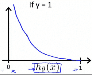
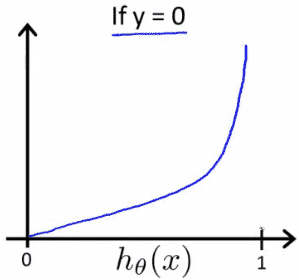
Instead, our cost function for logistic regression looks like:\[
\begin{align}& J(\theta) = \dfrac{1}{m} \sum_{i=1}^m \mathrm{Cost}(h_\theta(x^{(i)}),y^{(i)}) \newline & \mathrm{Cost}(h_\theta(x),y) = -\log(h_\theta(x)) \; & \text{if y = 1} \newline & \mathrm{Cost}(h_\theta(x),y) = -\log(1-h_\theta(x)) \; & \text{if y = 0}\end{align}
\]

• Logistic regression cost function \[
  \begin{align*}
  & \mathrm{Cost}(h_\theta(x),y) = 0 \text{ if } h_\theta(x) = y \newline
  & \mathrm{Cost}(h_\theta(x),y) \rightarrow \infty \text{ if } y = 0 \; \mathrm{and} \; h_\theta(x) \rightarrow 1 \newline
  & \mathrm{Cost}(h_\theta(x),y) \rightarrow \infty \text{ if } y = 1 \; \mathrm{and} \; h_\theta(x) \rightarrow 0 \newline \end{align*}
  \]

If our correct answer ‘y’ is 0, then the cost function will be 0 if our hypothesis function also outputs 0. If our hypothesis approaches 1, then the cost function will approach infinity.

If our correct answer ‘y’ is 1, then the cost function will be 0 if our hypothesis function outputs 1. If our hypothesis approaches 0, then the cost function will approach infinity.

Note that writing the cost function in this way guarantees that J(θ) is convex for logistic regression.

Simplified Cost function and Gradient Decent

We can compress our cost function’s two conditional cases into one case:

\[
\mathrm{Cost}(h_\theta(x),y) = – y \; \log(h_\theta(x)) – (1 – y) \log(1 – h_\theta(x))
\]

Notice that when y is equal to 1, then the second term \((1-y)\log(1-h_\theta(x))\) will be zero and will not affect the result. If y is equal to 0, then the first term \(-y \log(h_\theta(x))\) will be zero and will not affect the result.

We can fully write out our entire cost function as follows:

• Logistic regression cost function$$
  \begin{align*}
  J(\theta)&=\frac1m\sum_{i=1}^m Cost(h_\theta(x^{(i)},y^{(i)})\\
  &=-\frac1m \sum_{i=1}^m [y^{(i)} \log h_\theta(x^{(i)})+(1-y^{(i)})\log(1-h_\theta(x^{(i)}))]
  \end{align*}
  $$
  • To fit parameters \(\theta\):$$\min_\theta J(\theta)$$
  • To make a prediction given new x:$$
    h_\theta(x)=\frac{1}{1+e^{-\theta^Tx}}
    $$

A vectorized implementation is:\[
\begin{align} & h = g(X\theta)\newline & J(\theta) = \frac{1}{m} \cdot \left(-y^{T}\log(h)-(1-y)^{T}\log(1-h)\right) \end{align}
\]

Gradient Descent

• Remember that the general form of gradient descent is:$$
  \begin{align*}
  &Repeat:\{\\
  &\theta_j := \theta_j – \alpha \frac{\partial}{\partial \theta_j} J(\theta)\\
  &\}
  \end{align*}
  $$
• We can work out the derivative part using calculus to get:$$
  \begin{align*}
  &Repeat:\{\\
  &\theta_j := \theta_j – \frac{\alpha}{m}\sum_{i=1}^{m}(h_\theta(x^{(i)})-y^{(i)})x_j^{(i)}\\
  &\}
  \end{align*}
  $$
• A vectorized implementation is: $$
  \theta := \theta-\frac{\alpha}{m}X^T(g(X\theta)-\vec{y})
  $$
  

Advanced Optimization

• Optimization algorithm
  • Gradient descent
  • Conjugate gradient
  • BFGS
  • L-BFGS
• Advantages
  • \(\alpha\)をpickしなくてもいい
  • はやい
• Disadvantages
  • 複雑

Octave

evaluates the following two functions for a given input value θ:

$$ \begin{align*} & J(\theta) \newline & \dfrac{\partial}{\partial \theta_j}J(\theta)\end{align*}$$

function [jVal, gradient] = costFunction(theta)
  jVal = [...code to compute J(theta)...];
  gradient = [...code to compute derivative of J(theta)...];
end

octaveのfminunc()を利用

options = optimset('GradObj', 'on', 'MaxIter', 100);
initialTheta = zeros(2,1);
   [optTheta, functionVal, exitFlag] = fminunc(@costFunction, initialTheta, options);

Multiclass Classification

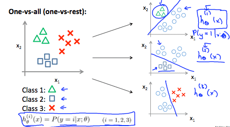
Multiclass Classification: One-vs-all

Now we will approach the classification of data when we have more than two categories. Instead of y = {0,1} we will expand our definition so that y = {0,1…n}.

Since y = {0,1…n}, we divide our problem into n+1 (+1 because the index starts at 0) binary classification problems; in each one, we predict the probability that ‘y’ is a member of one of our classes.

\[
\begin{align}& y \in \lbrace0, 1 … n\rbrace \newline& h_\theta^{(0)}(x) = P(y = 0 | x ; \theta) \newline& h_\theta^{(1)}(x) = P(y = 1 | x ; \theta) \newline& \cdots \newline& h_\theta^{(n)}(x) = P(y = n | x ; \theta) \newline& \mathrm{prediction} = \max_i( h_\theta ^{(i)}(x) )\newline\end{align}
\]

We are basically choosing one class and then lumping all the others into a single second class. We do this repeatedly, applying binary logistic regression to each case, and then use the hypothesis that returned the highest value as our prediction.

The following image shows how one could classify 3 classes:

To summarize:

• Train a logistic regression classifier \(h^{(i)}_\theta(x)\) for each class i to predict the probability that y=i.
• To make a prediction on a new x, pick the class i that maximizes \(h^{(i)}_\theta (x)\) \[
  \max_i( h_\theta ^{(i)}(x) )
  \]

(note)

• One-vs-all
  • 複数のクラス分け問題を、1つ対他の2クラスと置き換える
  • i: to predict the probability that y=i.
  • On a new input x to make a prediction, pick the class i that maximizes.

Solving the Problem of Overfitting

Problem of Overfitting

• underfitting, high bias
• overfitting, high variance
• Addressing overfitting
  • Reduce number of features.
    • manually select which features to keep.
    • Model selection algorithm (later in course).
  • Regularization
    • Keep all the features, but reduce magnitude/values of parameters \(\theta_j\).
    • Works well when we have a lot of features, each of which contributes a bit to predicting \(y\).

Cost function

If we have overfitting from our hypothesis function, we can reduce the weight that some of the terms in our function carry by increasing their cost.

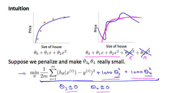
Say we wanted to make the following function more quadratic:

\(\theta_0 + \theta_1x + \theta_2x^2 + \theta_3x^3 + \theta_4x^4\)

We’ll want to eliminate the influence of \(\theta_3x^3\) and \(\theta_4x^4\). Without actually getting rid of these features or changing the form of our hypothesis, we can instead modify our cost function:

\(min_\theta\ \dfrac{1}{2m}\sum_{i=1}^m (h_\theta(x^{(i)}) – y^{(i)})^2 + 1000\cdot\theta_3^2 + 1000\cdot\theta_4^2\)​

We’ve added two extra terms at the end to inflate the cost of \(\theta_3\) and \(\theta_4\). Now, in order for the cost function to get close to zero, we will have to reduce the values of \(\theta_3\) and \(\theta_4\) to near zero. This will in turn greatly reduce the values of \(\theta_3x^3\) and \(\theta_4x^4\) in our hypothesis function. As a result, we see that the new hypothesis (depicted by the pink curve) looks like a quadratic function but fits the data better due to the extra small terms \(\theta_3x^3\) and \(\theta_4x^4\).

We could also regularize all of our theta parameters in a single summation as:\[
min_\theta\ \dfrac{1}{2m}\ \sum_{i=1}^m (h_\theta(x^{(i)}) – y^{(i)})^2 + \lambda\ \sum_{j=1}^n \theta_j^2
\]

The λ, or lambda, is the regularization parameter. It determines how much the costs of our theta parameters are inflated.

Using the above cost function with the extra summation, we can smooth the output of our hypothesis function to reduce overfitting. If lambda is chosen to be too large, it may smooth out the function too much and cause underfitting. Hence, what would happen if \(\lambda = 0\) or is too small ?

(note)

• Regularization
  • \(\theta\)を小さく保つことがスムーズな関数であることを意味する（e.g. 高次項の影響を最小化）
  • Regularization parameter: \(\lambda\)
  • $$
    J(\theta)=\frac{1}{2m}[\sum_{i=1}^m(h_\theta(x^{(i)})-y^{(i)})^2+\lambda\sum_{j=1}^n \theta_j^2]
    $$
  • \(\lambda\)を大きくすると、\(\theta_0\)以外がほぼゼロになる、といういうことは、直線でunderfittingしているのとほぼ同じ

Regularized Linear Regression

We can apply regularization to both linear regression and logistic regression. We will approach linear regression first.

• Gradient descent
  • We will modify our gradient descent function to separate out \(\theta_0\)​ from the rest of the parameters because we do not want to penalize \(\theta_0\)​.
  • Repeat{ $$
    \begin{align*}
    \theta_0 &:= \theta_0 – \alpha \frac1m \sum_{i-1}^m (h_\theta(x^{(i)})-y^{(i)})x_0^{(i)} \dots (j=0)\\
    \theta_j &:= \theta_j – \alpha \left[\frac1m \sum_{i-1}^m (h_\theta(x^{(i)})-y^{(i)})x_j^{(i)}+\frac{\lambda}{m}\theta_j\right] \dots (j=1,2,3,\dots,n)
    \end{align*}
    $$
    }
  • The term \(\frac{\lambda}{m}\theta_j\)​ performs our regularization. With some manipulation our update rule can also be represented as:
  • $$
    \theta_j := \theta_j(1 – \alpha \frac{\lambda}m) – \alpha \frac1m \sum_{i-1}^m (h_\theta(x^{(i)})-y^{(i)})x_j^{(i)}
    $$
  • The first term in the above equation, \(1 – \alpha\frac{\lambda}{m}\)​ will always be less than 1. Intuitively you can see it as reducing the value of \(\theta_j\)​ by some amount on every update. Notice that the second term is now exactly the same as it was before.
  • updateのたびにちょっとだけ縮める $$ 1 – \alpha \frac{\lambda}m >1$$

Normal equation

Now let’s approach regularization using the alternate method of the non-iterative normal equation.

To add in regularization, the equation is the same as our original, except that we add another term inside the parentheses:\[
\begin{align}& \theta = \left( X^TX + \lambda \cdot L \right)^{-1} X^Ty \newline& \text{where}\ \ L = \begin{bmatrix} 0 & & & & \newline & 1 & & & \newline & & 1 & & \newline & & & \ddots & \newline & & & & 1 \newline\end{bmatrix}\end{align}
\]

L is a matrix with 0 at the top left and 1’s down the diagonal, with 0’s everywhere else. It should have dimension (n+1)×(n+1). Intuitively, this is the identity matrix (though we are not including \(x_0\)​), multiplied with a single real number λ.

\[
\displaylines{
X=\begin{bmatrix}
(x^{(1)})^T\\
\vdots \\
(x^{(m)})^T
\end{bmatrix}\Bbb R^{m \times n+1}\\
y=\begin{bmatrix}
y^{(1)}\\
\vdots \\
y^{(m)}
\end{bmatrix} \Bbb R^{m}
}
\]

• Non-invertibility (optional/advanced)
  • Supporse \(m\leq n\)
  • $$
    \theta=(\underbrace{X^TX}_{\text{non-invertible}})^{-1}X^Ty
    $$
    • Octave: pinvをつかう
  • 正規化でinvertibleになる$$
    \displaylines{
    \text{If }\lambda\gt0\\
    \theta=(X^TX + \lambda \cdot L)^{-1}X^Ty
    }
    $$

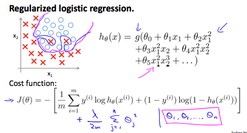
Regularized Logistic Regression

We can regularize logistic regression in a similar way that we regularize linear regression. As a result, we can avoid overfitting. The following image shows how the regularized function, displayed by the pink line, is less likely to overfit than the non-regularized function represented by the blue line:

• Logistic regression cost function$$
  \begin{align*}
  J(\theta)&=-\frac1m \sum_{i=1}^m [y^{(i)} \log h_\theta(x^{(i)})+(1-y^{(i)})\log(1-h_\theta(x^{(i)}))]
  \end{align*}
  $$
• We can regularize this equation by adding a term to the end:$$
  \begin{align*}
  J(\theta)&=-\frac1m \sum_{i=1}^m [y^{(i)} \log h_\theta(x^{(i)})+(1-y^{(i)})\log(1-h_\theta(x^{(i)}))]+\frac{\lambda}{2m}\sum_{j=1}^n \theta_j^2
  \end{align*}
  $$
  • The second sum, \(\sum_{j=1}^n \theta_j^2\) means to explicitly exclude the bias term, \(\theta_0\)
• Gradient descent
  • Repeat{ $$
    \begin{align*}
    \theta_0 &:= \theta_0 – \alpha \frac1m \sum_{i-1}^m (h_\theta(x^{(i)})-y^{(i)})x_0^{(i)} \dots (j=0)\\
    \theta_j &:= \theta_j – \alpha \left[\frac1m \sum_{i-1}^m (h_\theta(x^{(i)})-y^{(i)})x_j^{(i)}+\frac{\lambda}{m}\theta_j \right] \dots (j=1,2,3,\dots,n)
    \end{align*}
    $$
    }
  • Regularized Linear Regressionとの違いは、$$h_\theta(x)=\frac{1}{1+e^{-\theta^Tx}}$$

MATLAB code memo

cost function(normal)

h_theta_x = sigmoid(X * theta);
J = 1/m * sum(-y.* log(h_theta_x) - (1-y) .* log(1-h_theta_x));
grad = 1/m * sum((h_theta_x-y) .* X)';

cost function(regularized)

h_theta_x = sigmoid(X * theta);

cost = 1/m * sum(-y.* log(h_theta_x) - (1-y) .* log(1-h_theta_x));
theta_reg = [0; theta(2:size(theta))];
reg = lambda / (2 * m) * sum(theta_reg'*theta_reg);
J = cost+reg;

grad = 1/m * sum((h_theta_x-y) .* X)' + lambda / m * theta_reg;