[mathjax]
Machine Learning (Stanford University) の受講メモ
- 内容
- Neural network forward propagation
- Multiple classification using logistic regression and the one-vs-all technique
- メモ
- この講座だと、\(x_0\) としてb(ias)定義し、\(\Theta\)のDimensionを求めている。
- \(z=wx+b\)
- \( w.shape:(n^{[l]},n^{[l-1]})\)
- \( \Theta.shape:(s_{j+1},s_j+1)\): +1はbias
Motivations
Non-linear Hypotheses
Picture: feature N is too large.
Neurons and the Brain
Origins: Algorithms that try to mimic the brain. 80s-early 90s; popularity diminished in late 90s.
Recent resurgence: State-of-the-art technique for many applications.
- The “one learning algorithm” hypothesis
- Auditory cortex learns to see.
- Somatosensory cortex learns to see.
- Sensor representations in the brain
- Seeing with your tongue.
- Human echolocation (sonar).
- Haptic belt: Direction sense.
- Implanting a 3rd eye.
- センサーは脳のたいていの場所に繋げて、扱い方学習する
- コースではNNは人工知能のためではなく、機械学習の応用として扱う
Neural Networks
Model Representation I
Let’s examine how we will represent a hypothesis function using neural networks. At a very simple level, neurons are basically computational units that take inputs (dendrites) as electrical inputs (called “spikes”) that are channeled to outputs (axons). In our model, our dendrites are like the input features \(x_1\cdots x_n\), and the output is the result of our hypothesis function. In this model our \(x_0\) input node is sometimes called the “bias unit.” It is always equal to 1. In neural networks, we use the same logistic function as in classification, \(\frac{1}{1 + e^{-\theta^Tx}}\), yet we sometimes call it a sigmoid (logistic) activation function. In this situation, our “theta” parameters are sometimes called “weights”.
- Neurons in the brain
- Neuron model: Logistic unit
- \(x_0=1\): bias unit
- 便利だから
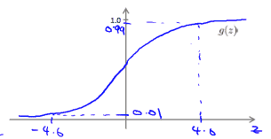
- \(g(z)\): Sigmoid(logistic)activation function.
- \(\theta\): weight
- \(x_0=1\): bias unit
- label
- \[
\begin{align*}& a_i^{(j)} = \text{“activation” of unit $i$ in layer $j$} \newline& \Theta^{(j)} = \text{matrix of weights controlling function mapping from layer $j$ to layer $j+1$}\end{align*}
\]
- \[
- one hidden layer
- \[
\begin{bmatrix}x_0 \newline x_1 \newline x_2 \newline x_3\end{bmatrix}\rightarrow\begin{bmatrix}a_1^{(2)} \newline a_2^{(2)} \newline a_3^{(2)} \newline \end{bmatrix}\rightarrow h_\theta(x)
\]
- \[
- The values for each the “activation” nodes
- \[
\begin{align*} a_1^{(2)} = g(\Theta_{10}^{(1)}x_0 + \Theta_{11}^{(1)}x_1 + \Theta_{12}^{(1)}x_2 + \Theta_{13}^{(1)}x_3) \newline a_2^{(2)} = g(\Theta_{20}^{(1)}x_0 + \Theta_{21}^{(1)}x_1 + \Theta_{22}^{(1)}x_2 + \Theta_{23}^{(1)}x_3) \newline a_3^{(2)} = g(\Theta_{30}^{(1)}x_0 + \Theta_{31}^{(1)}x_1 + \Theta_{32}^{(1)}x_2 + \Theta_{33}^{(1)}x_3) \newline h_\Theta(x) = a_1^{(3)} = g(\Theta_{10}^{(2)}a_0^{(2)} + \Theta_{11}^{(2)}a_1^{(2)} + \Theta_{12}^{(2)}a_2^{(2)} + \Theta_{13}^{(2)}a_3^{(2)}) \newline \end{align*}
\] - This is saying that we compute our activation nodes by using a 3×4 matrix of parameters. We apply each row of the parameters to our inputs to obtain the value for one activation node. Our hypothesis output is the logistic function applied to the sum of the values of our activation nodes, which have been multiplied by yet another parameter matrix \(\Theta^{(2)}\) containing the weights for our second layer of nodes.
- \[
- The dimensions of these matrices of weights
- If network layer \( j \) unit \( s_j \) to layer \( j+1 \) unit \( s_{j+1} \) will be of dimension:\[
\Theta^{(j)}\in\Bbb R^{( s_{j+1} \times (s_j + 1) )}
\] - Example: If layer 1 has 2 input nodes and layer 2 has 4 activation nodes. Dimension of \(\Theta^{(1)}\) is going to be 4×3 where \(s_j = 2\) and \(s_{j+1} = 4\), so \(s_{j+1} \times (s_j + 1) = 4 \times 3\).
- If network layer \( j \) unit \( s_j \) to layer \( j+1 \) unit \( s_{j+1} \) will be of dimension:\[
Model Representation II
- Forward propagation: Vectorized implementation
- In this section we’ll do a vectorized implementation of the above functions. We’re going to define a new variable \(z_k^{(j)}\) that encompasses the parameters inside our g function. In our previous example if we replaced by the variable z for all the parameters we would get:\[
\begin{align*}a_1^{(2)} = g(z_1^{(2)}) \newline a_2^{(2)} = g(z_2^{(2)}) \newline a_3^{(2)} = g(z_3^{(2)}) \newline \end{align*}
\]
- layer j=2 and node k, the variable z will be: \[
z_k^{(2)} = \Theta_{k,0}^{(1)}x_0 + \Theta_{k,1}^{(1)}x_1 + \cdots + \Theta_{k,n}^{(1)}x_n
\] - Vector representation of x and z^j\[
\begin{align*}x = \begin{bmatrix}x_0 \newline x_1 \newline\cdots \newline x_n\end{bmatrix} &z^{(j)} = \begin{bmatrix}z_1^{(j)} \newline z_2^{(j)} \newline\cdots \newline z_n^{(j)}\end{bmatrix}\end{align*}
\] - \[
z^{(j)} = \Theta^{(j-1)}a^{(j-1)}
\] - We are multiplying our matrix \(\Theta^{(j-1)}\) with dimensions \(s_j\times (n+1)\) (where \(s_j\) is the number of our activation nodes) by our vector \(a^{(j-1)}\) with height (n+1). This gives us our vector \(z^{(j)}\) with height \(s_j\). Now we can get a vector of our activation nodes for layer j as follows:\[
a^{(j)} = g(z^{(j)})
\] - We can then add a bias unit (equal to 1) to layer j after we have computed \(a^{(j)}\). This will be element \(a_0^{(j)}\) and will be equal to 1. To compute our final hypothesis, let’s first compute another z vector:\[
z^{(j+1)} = \Theta^{(j)}a^{(j)}
\] - We get this final z vector by multiplying the next theta matrix after \(\Theta^{(j-1)}\) with the values of all the activation nodes we just got. This last theta matrix \(\Theta^{(j)}\) will have only one row which is multiplied by one column \(a^{(j)}\) so that our result is a single number. We then get our final result with:\[
h_\Theta(x) = a^{(j+1)} = g(z^{(j+1)})
\]
- In this section we’ll do a vectorized implementation of the above functions. We’re going to define a new variable \(z_k^{(j)}\) that encompasses the parameters inside our g function. In our previous example if we replaced by the variable z for all the parameters we would get:\[
Applications
Examples and Intuitions I
- Function: x1 and x2 then true;
- The graph of our functions will look like:\[
\begin{align*}\begin{bmatrix}x_0 \newline x_1 \newline x_2\end{bmatrix} \rightarrow\begin{bmatrix}g(z^{(2)})\end{bmatrix} \rightarrow h_\Theta(x)\end{align*}
\] - first matrix:\[
\Theta^{(1)} =\begin{bmatrix}-30 & 20 & 20\end{bmatrix}
\] - \[
\begin{align*}& h_\Theta(x) = g(-30 + 20x_1 + 20x_2) \newline \newline & x_1 = 0 \ \ and \ \ x_2 = 0 \ \ then \ \ g(-30) \approx 0 \newline & x_1 = 0 \ \ and \ \ x_2 = 1 \ \ then \ \ g(-10) \approx 0 \newline & x_1 = 1 \ \ and \ \ x_2 = 0 \ \ then \ \ g(-10) \approx 0 \newline & x_1 = 1 \ \ and \ \ x_2 = 1 \ \ then \ \ g(10) \approx 1\end{align*}
\]
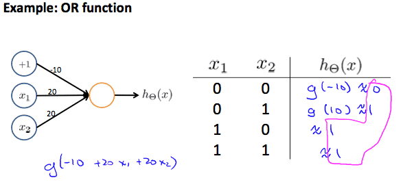
So we have constructed one of the fundamental operations in computers by using a small neural network rather than using an actual AND gate. Neural networks can also be used to simulate all the other logical gates. The following is an example of the logical operator ‘OR’, meaning either \(x_1\) is true or \(x_2\) is true, or both:
Examples and Intuitions II
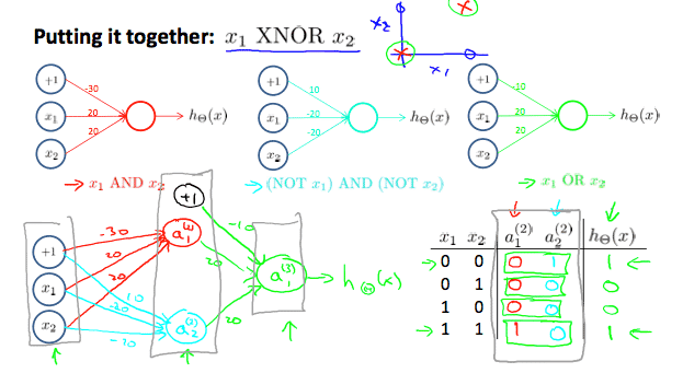
- FunctionをAND,NOR,ORとして直感的な理解を
Multiclass Classification
To classify data into multiple classes, we let our hypothesis function return a vector of values. Say we wanted to classify our data into one of four categories. We will use the following example to see how this classification is done. This algorithm takes as input an image and classifies it accordingly:
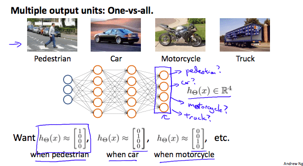
- We can define our set of resulting classes as y:\[
y^{(i)}=\begin{bmatrix}1\\0\\0\\0\end{bmatrix}, \begin{bmatrix}0\\1\\0\\0\end{bmatrix}, \begin{bmatrix}0\\0\\1\\0\end{bmatrix}, \begin{bmatrix}0\\0\\0\\1\end{bmatrix}
\] - Our final hypothesis function setup:\[
\begin{bmatrix}x_0\\x_1\\x_2\\x_3\end{bmatrix}\rightarrow \begin{bmatrix}a_0^{[2]}\\ a_1^{[2]}\\a_2^{[2]}\\ a_3^{[2]}\end{bmatrix} \rightarrow \begin{bmatrix} a_0^{[3]}\\ a_1^{[3]} \\ a_2^{[3]}\\ a_3^{[3]}\end{bmatrix} \rightarrow\dots\rightarrow\begin{bmatrix}h_\Theta (x)_1\\ h_\Theta (x)_2 \\ h_\Theta (x)_3 \\ h_\Theta (x)_4 \end{bmatrix}
\] - Our resulting hypothesis for one set of inputs may look like:\[
h_\Theta(x) =\begin{bmatrix}0 \newline 0 \newline 1 \newline 0 \newline\end{bmatrix}
\]