Why sequence models
Examples of sequence data
- Speech recognition
- x: wave🌊
- y: “The quick brown fox jumped over the lazy dog.”
- Music generation
- \( \emptyset \)
- ♬🎼
- Sentiment classification
- “There is nothing to like in this movie.”
- ★☆☆☆☆
- DNA sequence analysis
- AGCCCCTGTGAGGAACTAG
- AGCCCCTGTGAGGAACTAG
- Machine translation
- Voulez-vous chanter avec moi?
- Do you want to sing with me?
- Video activity recognition
- 📺
- Running
- Name entity recognition
- Yesterday, Harry Potter met Hermione Granger.
- Yesterday, Harry Potter met Hermione Granger.
Notation
Motivating example
x: Harry Potter and Hermione Granger invented a new spell.
y: 1 1 0 1 1 0 0 0 0
\[
x^{<1>}x^{<2>}x^{<3>} \dots x^{<t>} \dots x^{<9>}\\
T_X=9\\
y^{<1>}y^{<2>}y^{<3>} \dots y^{<t>} \dots y^{<9>}\\
T_y=9\\
X^{(i)<t>} T_X^{(i)}\\
y^{(i)<t>} T_y^{(i)}
\]
- The parentheses represent the training example.
- The brackets represent the word.
Representing words
- one-hot representation
- 10000 words: small
- commercial size: 30000 to 50000 words
\[
\displaylines{
x: \text{Harry Potter and Hermione Granger invented a new spell.}\\
x^{<1>}x^{<2>}x^{<3>} \dots x^{<t>} \dots x^{<9>}\\
\overbrace{
\begin{bmatrix}
a\\
\vdots \\
aaron\\
\vdots \\
<unk>\\
\vdots \\
harry\\
\vdots \\
potter\\
\end{bmatrix}}^{Vocabulary}
\overbrace{
\begin{bmatrix}
0\\
\vdots \\
0\\
\vdots \\
0\\
\vdots \\
1\\
\vdots \\
0\\
\end{bmatrix}}^{X^{<1>}}
\overbrace{
\begin{bmatrix}
0\\
\vdots \\
0\\
\vdots \\
0\\
\vdots \\
0\\
\vdots \\
1\\
\end{bmatrix}}^{X^{<2>}}
\dots
\overbrace{
\begin{bmatrix}
0\\
\vdots \\
0\\
\vdots \\
1\\
\vdots \\
0\\
\vdots \\
0\\
\end{bmatrix}}^{X^{<t>}}
\dots
\overbrace{
\begin{bmatrix}
1\\
\vdots \\
0\\
\vdots \\
0\\
\vdots \\
0\\
\vdots \\
0\\
\end{bmatrix}}^{X^{<9>}}
}
\]
<UNK>: Unkonwn Word token
Recurrent Neural Network Model
Why not a standard network?
\[
\begin{vmatrix}
x^{<1>}\\ x^{<2>}\\ \vdots \\x^{<T_x>}
\end{vmatrix}
\rightarrow
\begin{vmatrix}
\fc
\end{vmatrix}
\rightarrow
\begin{vmatrix}
\fc
\end{vmatrix}
\rightarrow
\begin{vmatrix}
y^{<1>}\\ y^{<2>}\\ \vdots \\y^{<T_y>}
\end{vmatrix}
\]
- Problems
- Inputs, outputs can be different length in different examples.
- Doesn’t share features learned across different positions of text.
Recurrent Neural Networks
| \(\hat{y}^{<1>}\\\uparrow \color{red}{W_{ya}}\) | \(\hat{y}^{<2>}\\\uparrow \color{red}{W_{ya}}\) | \(\hat{y}^{<3>}\\\uparrow \color{red}{W_{ya}}\) | \(\hat{y}^{<T_y>}\\\uparrow \color{red}{W_{ya}}\) | ||||
| \(a^{<0>}\rightarrow \\\color{red}{W_{aa}}\) | \(\boxed{\circ\\\circ\\\circ\\\vdots\\\circ}\) | \(a^{<1>}\rightarrow\\\color{red}{W_{aa}}\) | \(\boxed{\circ\\\circ\\\circ\\\vdots\\\circ}\) | \(a^{<2>}\rightarrow\\\color{red}{W_{aa}}\) | \(\boxed{\circ\\\circ\\\circ\\\vdots\\\circ}\) | \(\dots a^{<T_x-1>}\rightarrow\\\color{red}{W_{aa}}\) | \(\boxed{\circ\\\circ\\\circ\\\vdots\\\circ}\) |
| \(\uparrow \color{red}{W_{ax}}\\x^{<1>}\) | \(\uparrow \color{red}{W_{ax}} \\x^{<2>}\) | \(\uparrow \color{red}{W_{ax}}\\x^{<3>}\) | \(\uparrow \color{red}{W_{ax}}\\x^{<T_x>}\) |
\(a^{<0>}\): vector of zero
- He said, “Teddy Roosevelt was a great President.”
- He said, Teddy bears are on safe!
- Problem:
- given just the first three words is not possible to know for sure whether the word Teddy is part of a person’s name.
- You can’t tell the defference if you look only at the first three words.
- The prediction at a uses inputs or uses information from the inputs earlier in the sequence but not information later in the sequence.
- bi-directional recurrent neural networks (BRNN)双方向再帰型ニューラルネットワーク
Forward Propagation
\[
\eqalign{
a^{<0>}&=\vec{0}\\
a^{<1>}&=g(W_{aa}a^{<0>}+W_{ax}x^{<1>}+b_a) \leftarrow \tanh|LeLU\\
\hat{y}^{<1>}&=g(W_{ya}a^{<1>}+b_y) \leftarrow sigmoid\\
a^{<t>}&=g(W_{aa}a^{<t-1>}+W_{ax}x^{<t>}+b_a)\\
\hat{y}^{<t>}&=g(W_{ya}a^{<t>}+b_y)
}
\]
Simplified RNN notation
\[
\eqalign{
a^{<t>}&=g(\underbrace{W_{aa}}_{(100,100)}a^{<t-1>}+\underbrace{W_{ax}}_{(100,10000)}x^{<t>}+b_a)\\
\hat{y}^{<t>}&=g(W_{ya}a^{<t>}+b_y)\\
\color{blue}{\hat y ^{<t>}} &= \color{blue}{g(W_y a^{<t>}+b_y)\dots \star}
}
\]
\[
\displaylines{
\color{blue}{
a^{<t>}=g(W_a }\color{purple}{\boxed{\color{bule}{[a^{<t-1>},x^{<t>}]}}}+b_a)\dots \star\\
\color{blue}{
(100) \{ [\underbrace{W_{aa}}_{(100)} \vdots \underbrace{W_{ax}}_{(10000)}]=\underbrace{W_a}_{(100,10100)}
}
\\
\color{purple}{
[a^{<t-1>},x^{<t>}] =\left[ \frac{a^{<t-1>}}{x^{<t>}} \right] \}\scriptsize{(100+10000=10100)}
}\\
\color{green}{
[W_{aa} \vdots W_{ax}] \left[ \frac{a^{<t-1>}}{x^{<t>}} \right] = W_{aa}a^{<t-1>}+W_{ax}x^{<t>}
}\\
}
\]
- Advantage of this notation
- rather than carrying around two parameter matrices, Waa and Wax.
Backpropagation through time
Forward propagation and backpropagation
| \(L^{<1>}\) | \(L^{<2>}\) | \(L^{<T_y>}\) | |||||||
| ↑↓ | ↑↓ | ↑↓ | |||||||
| \(\color{green}{W_yb_y}\) | \(\hat y^{<1>}\) | \(\hat y^{<2>}\) | \(\hat y^{<T_y>}\) | ||||||
| ↑↓ | ↑↓ | ↑↓ | |||||||
| \(\color{green}{W_ab_a}\) | \(a^{<0>}\) | → | \(a^{<1>}\) | ← → | \(a^{<2>}\) | ← → | … | ← → | \(a^{<T_x>}\) |
| ↑ | ↑ | ↑ | |||||||
| \(x^{<1>}\) | \(x^{<2>}\) | … | \(x^{<T_x>}\) |
standard logistic regression loss (cross entropy loss)
\[
\eqalign{
L^{<t>}(\hat y^{<t>},y^{<t>})&=-y^{<t>}\log \hat y^{<t>}-(1- y^{<t>})\log(1-\hat y^{<t>})\\
L(\hat y,y)&=\sum_{t=1}^{T} L^{<t>}(\hat y^{<t>},y^{<t>})
}
\]
Different types of RNNs
\(T_x, T_y\) : different length problem
The Unreasonable Effectiveness of Recurrent Neural Networks
Examples of RNN architectures
- Image classification(input an image and output a label)
- one-to-one
- same
- many-to-many(same length)
- Sentiment classification / Gender recognition from speech
- x=text
- y=0/1
- many-to-one
- Music generation
- x->y1,y2,y3
- one-to-many
- Machine translation(English to French)
- many-to-many(encoder to decoder)
Summary of RNN types
Language model and sequence generation
What is language modelling?
- Speech recognition(which tells)
- The apple and pair salad.
- The apple and pear salad.
- (Probability)
- P(The apple and pair salad) = 3.2 x 10^-13
- P(The apple and pear salad) = 5.7 x 10^-10
- P(sentence) = ?
- P(y^<1>,y^<2>,…,y^<Ty>)
Language modelling with an RNN
- Training set: large corpus of english text.
- Cats average 15 hours of sleep a day.<EOS>
- y^<1>,y^<2>,…<EOS>
- The Egyptian Mau is a bread of cat.<EOS>
- <UNK>: unknown words
- corpus
- NLP terminology that just means a large body or a very large set of english text of english sentences.
- EOS
- End of Sentence
- ‘.’
- can add the period to your vocabulary as well
- UNK
- Unknown words replace with a unique token called UNK.
RNN Models
Cat average 15 hours of sleep a day.<EOS>
\[
\eqalign{
L(\hat y^{<t>}, y^{<t>}) &= -\sum_i y_i^{<t>} \log \hat y_i^{<t>}\\
L &= \sum_i L^{<t>}(\hat y^{<t>},y^{<t>})\\
P(y^{<1>},y^{<2>},y^{<3>})
&= P(y^{<1>})P(y^{<2>}|y^{<1>})P(y^{<3>}|y^{<1>},y^{<2>})
}
\]
Sampling novel sequences
Sampling a sequence from a trained RNN
- Training
- Sampling
- \( a^{<0>}=0, x^{<1>}=0\)
- softmax probability over possible outputs.
- softmax distribution
- \( P(a)P(aaron)\dots P(zulu)P(<unk>) \)
- np.random.choice: sampling function
- keep sampling until generate EOS token.
- this is how you would generate a randomly chosen sentence from your RNN language model.
- \( a^{<0>}=0, x^{<1>}=0\)
Character-lebel language model
- Vocabulary = [a, aaron, …, zulu, <UNK>]
- Vocabulary = [a, b, c, …,z, _, ., :,…,0, 1,…, A, B,…Z]
- pros
- You dont ever have to worry about unknown word tokens.
- cons
- You end up with much longer sequences.
- Just more computationally expensive to train.
Sequence generation
News and Shakespeare
If the model was trained on news articles, then it generates texts like that shown on the left. And this looks vaguely like news text, not quite grammatical, but maybe sounds a little bit like things that could be appearing news, concussion epidemic to be examined.
Vanishing gradients with RNNs
A basic RNN algorithm is that it runs into vanishing gradient problems.
- The cat, which already ate…,was full.
- The cats, which …………., were full.
\[
x\rightarrow
{\color{red}\fc}\rightarrow
{\color{red}\fc}\rightarrow
\fc\rightarrow
\fc\rightarrow
\fc\rightarrow
\fc\rightarrow
\hat y
\]
Very deep neural network say, 100 layers or even much deeper than you would carry out forward prop, from left to right and then back prop then the gradient from just output y would have a very hard time propagating back to affect the weights of these earlier layers, to affect the computations in the earlier layers.
An RNN has similar problem, because the basic RNN model has many local influences, meaning that the output \(\hat y^{<3>}\) is mainly influenced by calues close to \(x^{<1>}…x^{<3>}\)
Gated Recurrent Unit (GRU)
RNN unit
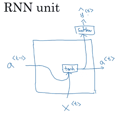
\[
a^{<t>}=\underbrace{g}_{\tanh}(W_a [a^{<t-1>},x^{<t>}]+b_a)
\]
GRU(simplified)
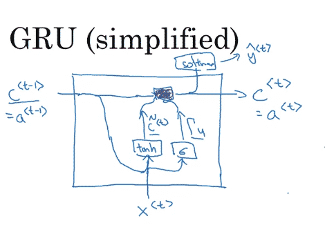
\[
\eqalign{
c&=\text{memory cell}\\
c^{<t>}&=a^{<t>}\\
\tilde{c}^{<t>}&=\tanh (W_c[c^{<t>},x^{<t>}]+b_c)\\
\color{green}{\Gamma_u}&=\sigma(W_u[c^{<t>},x^{<t>}]+b_u) \dots \text{update}\\
\color{green}{c^{<t>}}&=\Gamma_u \ast \tilde{c}^{<t>}+(1-\underbrace{\Gamma_u}_{0.0000001}) \ast \color{green}{c^{<t-1>}}
}
\]
The cat, which already ate …, was full.
cat:\(\Gamma_u=1, C^{<t>}=1\)
which:\(\Gamma_u=0\)
already:\(\Gamma_u=0\)
ate:\(\Gamma_u=0\)
was:\(\Gamma_u=1\)
- paper
Full GRU
\[
\eqalign{
\tilde{c}^{<t>}&=\tanh (W_c[\Gamma_r \ast c^{<t-1>},X^{<t>}]+b_c)\\
\Gamma_u&=\sigma(W_u[c^{<t-1>},x^{<t>}]+b_u)\\
\Gamma_r&=\sigma(W_r[c^{<t-1>},x^{<t>}]+b_r)\\
c^{<t>}&=\Gamma_u \ast \tilde{c}^{<t>}+(1- \Gamma_u) \ast c^{<t-1>}
}
\]
Long Short Term Memory (LSTM)
GRU and LSTM
GRU
\[
\eqalign{
\tilde{c}^{<t>}&=\tanh (W_c[\Gamma_r \ast c^{<t-1>},X^{<t>}]+b_c)\\
\Gamma_u&=\sigma(W_u[c^{<t-1>},x^{<t>}]+b_u)\\
\Gamma_r&=\sigma(W_r[c^{<t-1>},x^{<t>}]+b_r)\\
c^{<t>}&=\Gamma_u \ast \tilde{c}^{<t>}+\underbrace{(1- \Gamma_u)}_{\Gamma_f} \ast c^{<t-1>}\\
a^{<t>}&=c^{<t>}
}
\]
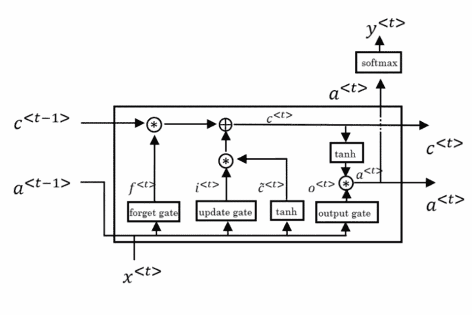
LSTM
\[
\eqalign{
\tilde{c}^{<t>}&=\tanh (W_c[a^{<t-1>},X^{<t>}]+b_c)\\
\Gamma_u&=\sigma(W_u[a^{<t-1>},x^{<t>}]+b_u) \dots \text{update}\\
\Gamma_f&=\sigma(W_f[a^{<t-1>},x^{<t>}]+b_f) \dots \text{forgot}\\
\Gamma_o&=\sigma(W_o[a^{<t-1>},x^{<t>}]+b_o) \dots \text{output}\\
c^{<t>}&=\Gamma_u \ast \tilde{c}^{<t>}+ \Gamma_f \ast c^{<t-1>}\\
a^{<t>}&=\Gamma_o \ast \tanh c^{<t>}
}
\]
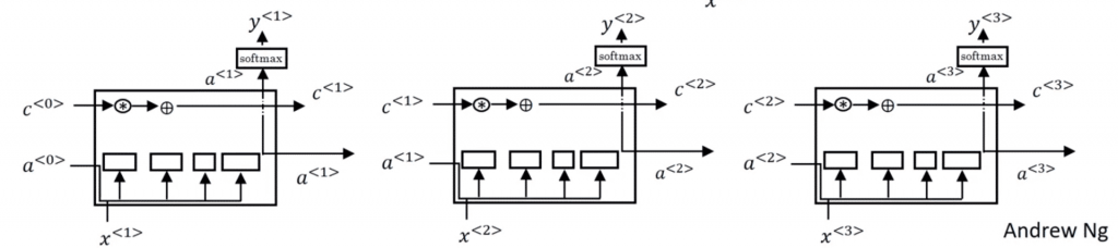
LSTM in pictures

tikz is so hard😱
Bidirectional RNN
Getting information from the future
- Advantage
- RNN and GRU or LSTM and is able to make predictions anywhere even in the middle of a sequence by taking into account information potentially from the entire sequence.
- Disadvantage
- You need the entire sequence of data before you can make predictions anywhere.
Deep RNNs
Deep RNN example
\[
a^{[2]<3>}=g(W_a^{[2]} [a^{[2]<2>},a^{[1]<3>}] + b_a^{[3]})
\]
Programming assignments
Building your Recurrent Neural Network – Step by Step
Notation:
- Superscript \([l]\) denotes an object associated with the \(l^{th}\) layer.
- Superscript \((i)\) denotes an object associated with the \(i^{th}\) example.
- Superscript \(⟨t⟩\) denotes an object at the \(t^{th}\) time-step.
- Subscript \(i\) denotes the \(i^{th}\) entry of a vector.
Example:
- \(a_5^{(2)[3]<4>}\) denotes the activation of the 2nd training example (2), 3rd layer [3], 4th time step , and 5th entry in the vector.
Character level language model – Dinosaurus Island
By completing this assignment you will learn:
- How to store text data for processing using an RNN
- How to synthesize data, by sampling predictions at each time step and passing it to the next RNN-cell unit
- How to build a character-level text generation recurrent neural network
- Why clipping the gradients is important
Improvise a Jazz Solo with an LSTM Network
You will learn to:
- Apply an LSTM to music generation.
- Generate your own jazz music with deep learning.